A step by step guide to Caffe

• Updates 05/2018

Although I’ve always appreciated views on my posts, as of 05/2018, I don’t think this post is relevant anymore. Deep learning has evolved with plenty of newer and much easier to use frameworks (Tensorflow, Caffe 2, etc.), so unless there’s a particular reason you have to use the original Caffe, browse other options before reading on.

• Intro

Caffe is a great and very widely used framework for deep learning, offers a vast collection of out-of-the-box layers and an amazing “model zoo”, however, it’s also famous for its lack of documentation.

After playing around with it for a few days, I felt that it would be great to share what I did to get everything up and running, especially some small hacks that I had to hunt around to get. I think it could well serve as a tutorial.

Before we get started, I strongly recommend going through This Course to get a theoretical primer about convolutional neural networks. The course has a great tutorial on Caffe as well, although it’s somewhat less detailed.

Now let’s get started.

• Get a desktop with a nice GPU!

Although most deep learning platforms can be run on CPU, it’s in general much slower. My personal experience is around 50-100 times slower, and I timed it once: 160 images per 35 seconds versus 5120 images in 26 seconds.

Up to this point I still think building a PC with a decent GPU is the best option (more flexible on IDE’s, flexible time of computation etc.), but if you don’t like to spend money on hardware, you can also use AWS or Terminal.com instead.

I found this great blog post on GPU selections. Take a look if you are wondering which GPU to buy.

• Install Caffe

The official documentation of Caffe has a pretty detailed instruction on installing Caffe here; they also provided a few platform specific step by step tutorials (e.g. here). Currently Ubuntu is best supported.

Thanks to the life saving apt-get install command, I was able to install most of the dependencies effortlessly. The Caffe package itself, however, needs to be compiled locally, some prior knowledge about make would help (not recommended to use the cmake script, it caused some issue for me).

• Data Preparation

Caffe is a high performance computing framework, to get more out of its amazing GPU accelerated training, you certainly don’t want to let file I/O slow you down, which is why a database system is normally used. The most common option is to use lmdb.

If you don’t have experience with database systems, basically lmdb will be a huge file on your computer once you finished data preparation. You can query any file from it using a scripting language, and reading big chunks of data from it is much faster can reading a file.

Caffe has a tool convert_imageset to help you build lmdb from a set of images. Once you build your Caffe, the binary will be under /build/tools. There’s also a bash script under /caffe/examples/imagenet that shows how to use convert_imageset.

You can also check out my recent post on how to write images into lmdb using Python.

Either way, once you are done, you’ll get two folders like below. The data.mdb files will be very large, that’s where your images went.

train_lmdb/
  -- data.mdb
  -- lock.mdb
val_lmdb/
  -- data.mdb
  -- lock.mdb

• Setting up the model and the solver

Caffe has a very nice abstraction that separates neural network definitions (models) from the optimizers (solvers). A model defines the structure of a neural network, while a solver defines all information about how gradient descent will be conducted.

A typical model looks like this (note that the lmdb files we generated are specified here!):

# train_val.prototxt
name: "MyModel"
layer {
  name: "data"
  type: "Data"
  top: "data"
  top: "label"
  include {
    phase: TRAIN
  }
  transform_param {
    mirror: false
    crop_size: 227
    mean_file: "data/train_mean.binaryproto" # location of the training data mean
  }
  data_param {
    source: "data/train_lmdb" # location of the training samples
    batch_size: 128 # how many samples are grouped into one mini-batch
    backend: LMDB
  }
}
layer {
  name: "data"
  type: "Data"
  top: "data"
  top: "label"
  include {
    phase: TEST
  }
  transform_param {
    mirror: false
    crop_size: 227
    mean_file: "data/train_mean.binaryproto"
  }
  data_param {
    source: "data/val_lmdb" # location of the validation samples
    batch_size: 50
    backend: LMDB
  }
}
layer {
  name: "conv1"
  type: "Convolution"
  bottom: "data"
  top: "conv1"
  param {
    lr_mult: 0.01
    decay_mult: 1
  }
  param {
    lr_mult: 0.01
    decay_mult: 0
  }
  convolution_param {
    num_output: 96
    kernel_size: 11
    stride: 4
    weight_filler {
      type: "gaussian"
      std: 0.01
    }
    bias_filler {
      type: "constant"
      value: 0
    }
  }
}
...
...
layer {
  name: "accuracy"
  type: "Accuracy"
  bottom: "fc8"
  bottom: "label"
  top: "accuracy"
  include {
    phase: TEST
  }
}
layer {
  name: "loss"
  type: "SoftmaxWithLoss"
  bottom: "fc8"
  bottom: "label"
  top: "loss"
}

This is actually a part of the AlexNet, you can find its full definition under /caffe/models/bvlc_alexnet.

If you use Python, install graphviz (install both the actuall graphviz using apt-get, and also the python package under the same name), you can use a script /caffe/python/draw_net.py to visualize the structure of your network and check if you made any mistake in the specification.

The resulting image will look like this:

Once the neural net is set up and hooked up with the lmdb files, you can write a solver.prototxt to specify gradient descent parameters.

net: "models/train_val.prototxt" # path to the network definition
test_iter: 200 # how many mini-batches to test in each validation phase
test_interval: 500 # how often do we call the test phase
base_lr: 1e-5 # base learning rate
lr_policy: "step" # step means to decrease lr after a number of iterations
gamma: 0.1 # ratio of decrement in each step
stepsize: 5000 # how often do we step (should be called step_interval)
display: 20 # how often do we print training loss
max_iter: 450000 
momentum: 0.9 
weight_decay: 0.0005 # regularization!
snapshot: 2000 # taking snapshot is like saving your progress in a game
snapshot_prefix: "models/model3_train_0422"
solver_mode: GPU
 

• Start training

So we have our model and solver ready, we can start training by calling the caffe binary:

caffe train \
  -gpu 0 \
  -solver my_model/solver.prototxt

note that we only need to specify the solver, because the model is specified in the solver file, and the data is specified in the model file.

We can also resume from a snapshot, which is very common (imaging if you are playing Assasin’s Creed and you need to start from the beginning everytime you quit game…):

caffe train \
    -gpu 0 \
    -solver my_model/solver.prototxt \
    -snapshot my_model/my_model_iter_6000.solverstate 2>&1 | tee log/my_model.log

or to fine tune from a trained network:

caffe train \
    -gpu 0 \
    -solver my_model/solver.prototxt \
    -weights my_model/bvlc_reference_caffenet.caffemodel 2>&1 | tee -a log/my_model.log

• Logging your performance

Optional: Try out NVIDIA DIGITS, a web based GUI for deep learning.

Once the training starts, Caffe will print training loss and testing accuracies in a frequency specified by you, however, it would be very useful to save those screen outputs to a log file so we can better visualize our progress, and that’s why we have those funky things in the code block above:

    ... 2>&1 | tee -a log/my_model.log

This half line of code uses a command called tee to “intercept” the data stream from stdout to the screen, and save it to a file.

Now the cool things: Caffe has a script (/caffe/tools/extra/parse_log.py) to parse log files and return two much better formatted files.

# my_model.log.train
NumIters,Seconds,LearningRate,loss
6000.0,10.468114,1e-06,0.0476156
6020.0,17.372427,1e-06,0.0195639
6040.0,24.237645,1e-06,0.0556274
6060.0,31.084703,1e-06,0.0244656
6080.0,37.927866,1e-06,0.0325582
6100.0,44.778659,1e-06,0.0131274
6120.0,51.62342,1e-06,0.0607449

# my_model.log.test
NumIters,Seconds,LearningRate,accuracy,loss
6000.0,10.33778,1e-06,0.9944,0.0205859
6500.0,191.054363,1e-06,0.9948,0.0191656
7000.0,372.292923,1e-06,0.9951,0.0186095
7500.0,583.508988,1e-06,0.9947,0.0211263
8000.0,806.678746,1e-06,0.9947,0.0192824
8500.0,1027.549856,1e-06,0.9953,0.0183917
9000.0,1209.650574,1e-06,0.9949,0.0194651

And with a little bit trick, you can automate the parsing process and combine it with curve plotting using a script like this:

# visualize_log.sh
python ~/caffe/tools/extra/parse_log.py my_model.log . # notice the dot in the end
gnuplot -persist gnuplot_commands

where gnuplot_commands is a file that stores a set of gnuplot commands.

# gnuplot_commands
set datafile separator ','
set term x11 0
plot '../my_model.log.train' using 1:4  with line,\
     '../my_model.log.test' using 1:5 with line
set term x11 1
plot '../my_model.log.test' using 1:4 with line

A sample result looks like this:

You can call the visualize_log.sh command at any time during training to check the progress. Even better, with more tweaks, we can make this plot live:

# visualize_log.sh
refresh_log() {
  while [true]; do
    python ~/caffe/tools/extra/parse_log.py ../my_model.log ../
    sleep 5 
  done
}
refresh_log & 
sleep 1
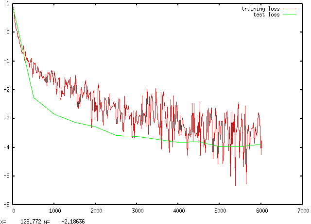
gnuplot gnuplot_commands

# gnuplot_commands
set datafile separator ','
plot '../model3_e-5.log.train' using 1:4  with line title 'training loss',\
     '../model3_e-5.log.test' using 1:5 with line title 'test loss'
pause 1
reread

There are a lot of things to talk about babysitting the training process, it’s out of the scope of this post though. The class notes from Stanford (here) has had it very well explained, take a look if you are interested.

The training process involves a search for multiple hyperparameters (as described in the solver), it’s actually quite complicated and requires certain level of experience to get the best training results.

• Deploy your model

Finally, after all the training process, we will like to use it in actual prediction. There are multiple ways of doing so, here I will describe the Pythonic way:

import numpy as np
import matplotlib.pyplot as plt
import sys
import caffe

# Set the right path to your model definition file, pretrained model weights,
# and the image you would like to classify.
MODEL_FILE = 'models/deploy.prototxt'
PRETRAINED = 'models/my_model_iter_10000.caffemodel'

# load the model
caffe.set_mode_gpu()
caffe.set_device(0)
net = caffe.Classifier(MODEL_FILE, PRETRAINED,
                       mean=np.load('data/train_mean.npy').mean(1).mean(1),
                       channel_swap=(2,1,0),
                       raw_scale=255,
                       image_dims=(256, 256))
print "successfully loaded classifier"

# test on a image
IMAGE_FILE = 'path/to/image/img.png'
input_image = caffe.io.load_image(IMAGE_FILE)
# predict takes any number of images,
# and formats them for the Caffe net automatically
pred = net.predict([input_image])

You’ll need a deploy.prototxt file to perform testing, which is quite easy to create, simply remove the data layers and add an input layer like this:

input: "data"
input_shape {
  dim: 10
  dim: 3
  dim: 227
  dim: 227
}

you can find a few examples in /caffe/model.

• That’s It!

This post describes how I conduct Caffe training, with some details explained here and there, hopefully it can give you a nice kickstart.

Caffe has a mixture of command line, Python and Matlab interfaces, you can definitely create a different pipeline that works best for you. To really learn about Caffe, it’s still much better to go through the examples under /caffe/examples/, and to checkout the official documentation, although it’s still not very complete yet.

Happy training!